Section Overview

Tutorial: 45 min

Objectives:

Learn basic modern fortran syntax and program structure.

Fortran Programming Basics

What we cover 

Fortran Program basics
Compile and run parallel Fortran code on Gadi
Live demo on profiling Fortran code with Gadi-supported tools

Prerequisites and setup 

Comfortable with the command line
Fortran compilers on Gadi: - GNU Fortran: gfortran through module gcc - Intel Fortran Classic: ifort through old intel-compiler/* modules - Intel Fortran ifx through intel-compiler-llvm/* modules - Parallel compiler wrapper mpif90 through openmpi or intel-mpi module.

Check installation:

gfortran --version
# or
ifort -V
# or
ifx -V

Compile and run 

Minimal commands:

gfortran -Wall -Wextra -O2 hello.f90 -o hello
./hello

On systems with multiple compilers, prefer explicit commands and flags. Use the .f90 extension for all modern Fortran source files (90/95/2003/2008).

Hello, Fortran 

Create hello.f90:

program hello
  implicit none
  print *, "Hello, Fortran 95!"
end program hello

Key idea: implicit none disables implicit typing and catches many bugs at compile time. Without it, the default sets undeclared variables to type real or integer based on their names.

Source form 

Free form source (.f90) is standard in F95.
Comments start with !.
Indentation is for humans, not the compiler, but keep it consistent.

Types and declarations 

Built-in numeric and logical types:

integer           :: i, n
real              :: x, y ! single precision
real(kind=8)  :: z ! double precision
real(kind=16) :: w ! long double precision as in C
logical           :: convergence
character(len=20) :: name

Use parameter for constants (much like const in C/C++):

integer, parameter :: wp = selected_real_kind(15,99) ! define work precision kind that has guaranteed 15 decimal digits with exponent range up to 99
real(kind=wp), parameter :: pi
pi = 3.1415926535_wp ! _wp enforces the wp kind

Operators (overview)

Arithmetic: + - * / **
Relational: == /= < <= > >=
Logical: .and. .or. .not.

Input and output 

List-directed I/O (simple and flexible):

integer :: n
print *, "Enter an integer:"
read  *, n
print *, "You entered:", n

Formatted I/O (controlled layout):

real :: x
x = 12.345
print '(A, F8.3)', "Value = ", x ! A for string, F8.3 for field width 8 with 3 decimals

If and case 

integer :: n
read *, n
if (n < 0) then
  print *, "negative"
else if (n == 0) then
  print *, "zero"
else
  print *, "positive"
end if

character(len=1) :: c
read *, c
select case (c)
case ('y','Y')
  print *, "yes"
case ('n','N')
  print *, "no"
case default
  print *, "unknown"
end select

Loops 

integer :: i, sum
sum = 0
do i = 1, 10
  sum = sum + i
end do
print *, "Sum 1..10 =", sum

Use exit to break, cycle to continue:

integer :: i
do i = 1, 1000
  if (i*i > 200) exit
  if (mod(i, 2) == 0) cycle
  print *, i
end do

1D arrays and array features 

Declaring arrays 

real :: a(5)              ! fixed-size
integer :: m, n
parameter (m=3, n=4)
real :: b(m, n)           ! 2D array, column-major

Array constructors and assignments 

 real :: x(5)
 x = (/ 1.0, 2.0, 3.0, 4.0, 5.0 /) ! x = [1.0, 2.0, 3.0, 4.0, 5.0] in fortran 2003.
 x = x * 2.0                ! whole-array operation
 print *, x

(/ ... /) and [ ... ] only create 1D arrays.

Multidimensional Arrays (Matrices)

Fortran is famously optimised for linear algebra and scientific computing. Unlike C or Python (where multidimensional arrays are often lists of lists), Fortran arrays are first-class citizens with built-in support for matrix arithmetic, slicing, and memory management.

Declaration and Rank 

In Fortran, the number of dimensions is called the Rank. Arrays can have up to 15 dimensions (in modern standards), though Rank-2 (Matrices) and Rank-3 (Cubes) are the most common.

Basic Syntax:

! Syntax: type :: variable_name(dim1, dim2, ...)

program matrix_demo
    implicit none

    ! A 3x3 Integer Matrix (Rank 2)
    integer :: matrix_A(3, 3)

    ! A 10x10x10 Real Cube (Rank 3)
    real :: tensor_B(10, 10, 10)

    ! Alternative declaration style (using dimension attribute)
    real, dimension(5, 5) :: matrix_C
end program matrix_demo

Column-Major Order (Crucial!)

Warning

Fortran is Column-Major. C and C++ are Row-Major.

This means that in memory, columns are stored contiguously. If you have a matrix A(2,2):

A(1,1) is stored first.
A(2,1) is stored second (Next row, same column).
A(1,2) is stored third.

Performance Tip: When looping over arrays, always iterate over the leftmost index (rows) first (innermost loop) and the rightmost index (columns) last (outermost loop).

! FAST (Correct Cache Usage)
do j = 1, 1000      ! Columns (Outer)
    do i = 1, 1000  ! Rows (Inner - changing fastest)
        A(i, j) = 0.0
    end do
end do

! SLOW (Cache Misses)
do i = 1, 1000
    do j = 1, 1000
        A(i, j) = 0.0
    end do
end do

Initialisation 

Because array constructors [...] create 1D arrays, you often use the intrinsic reshape function to mold data into a matrix.

integer :: A(2, 3)

! 1. Create a list of 6 numbers
! 2. Reshape it into 2 Rows and 3 Columns
! Note: Fills column 1, then column 2...
A = reshape( [1, 2, 3, 4, 5, 6], shape=[2,3] )

! Result:
! 1  3  5
! 2  4  6

Accessing Elements and Slicing 

Fortran indices start at 1 by default.

real :: A(4, 4)

! Access single element (Row 2, Col 3)
print *, A(2, 3)

Array Slicing (Sections) You can access whole rows, columns, or sub-matrices using the colon : operator.

! Whole Row 2
print *, A(2, :)

! Whole Column 3
print *, A(:, 3)

! Sub-matrix (Top-left 2x2 corner)
print *, A(1:2, 1:2)

! Stride: Rows 1 to 4, step 2 (Rows 1 and 3)
print *, A(1:4:2, :)

Matrix Arithmetic vs. Element-wise 

Standard operators in Fortran are Element-wise. For true linear algebra, you must use intrinsic functions.

real :: A(2,2), B(2,2), C(2,2)

! 1. Element-wise Multiplication
! C(i,j) = A(i,j) * B(i,j)
C = A * B

! 2. Matrix Multiplication (Linear Algebra)
! Row x Column dot products
C = matmul(A, B)

! 3. Transpose (Swap rows and cols)
C = transpose(A)

! 4. Summation
print *, sum(A)       ! Sum of all elements
print *, sum(A, dim=1) ! Sum down rows (returns a row vector)
print *, sum(A, dim=2) ! Sum across columns (returns a column vector)

Dynamic Allocation 

If you do not know the matrix size at compile time, use allocatable.

program dynamic_matrix
    implicit none
    integer, allocatable :: matrix(:, :) ! Rank 2, unknown size
    integer :: rows, cols, ierr

    print *, "Enter dimensions:"
    read *, rows, cols

    ! Allocate memory
    allocate( matrix(rows, cols) )

    ! Use the matrix
    matrix = 0
    print *, "Matrix size:", size(matrix)

    ! Free memory (Optional: happens automatically at end of program)
    deallocate(matrix)
end program dynamic_matrix

Summary Table 

Operation	Fortran Syntax	Meaning
Indexing	`A(i, j)`	Row `i`, Col `j`
Whole Row	`A(i, :)`	All columns in row `i`
Whole Col	`A(:, j)`	All rows in col `j`
Multiplication	`A * B`	Element-wise
Dot Product	`matmul(A, B)`	Matrix Math

Intrinsic procedures (basics)

real :: a(4), s
a = [ 1.0, -2.0, 3.0, -4.0 ]
s = sum(a)                 !  -2.0
print *, minval(a), maxval(a), sum(abs(a))

Fortran has many Intrinsic procesures. The most impressive ones are for array operations, and linear algebra. Saving you from writing big loops.

The most powerful concept in Fortran intrinsics is that most mathematical functions are Elemental.

This means they operate on a single number OR element-wise on an entire array.

The C Way:

// C requires a loop
for(int i=0; i<N; i++) {
    y[i] = sin(x[i]);
}

The Fortran Way:

! Fortran applies it to the whole array automatically
y = sin(x)

Intrinsic procedures (linear algebra)

These functions perform standard matrix math. They are typically optimised by the compiler to use SIMD instructions or call efficient BLAS libraries.

Procedure	Description
`matmul(matrix_a, matrix_b)`	Performs mathematical matrix multiplication (Row × Column).
`transpose(matrix)`	Transposes the matrix (swaps rows and columns).
`dot_product(vector_a, vector_b)`	Returns the scalar dot product of two 1D vectors.

Example:

real :: A(2, 2), B(2, 2), C(2, 2)

! 1. Element-wise multiplication (Not Matrix Math!)
C = A * B

! 2. True Matrix Multiplication
C = matmul(A, B)

! 3. Transpose
C = transpose(A)

Intrinsic procedures (reductions)

Reduction functions collapse a matrix into a scalar or a vector.

Most reduction functions accept an optional dim argument. If dim is omitted, the operation applies to the entire matrix.

dim=1: Operate down the rows (results in a row vector).
dim=2: Operate across the columns (results in a column vector).

Example:

integer :: M(2, 3) = reshape([1, 2, 3, 4, 5, 6], [2, 3])
! M looks like:
! 1  3  5
! 2  4  6

print *, sum(M)        ! Output: 21 (Total sum)
print *, sum(M, dim=1) ! Output: [3, 7, 11] (Sum of cols)
print *, sum(M, dim=2) ! Output: [9, 12]    (Sum of rows)

Intrinsic procedures (location querying)

Instead of finding the value of the maximum element, these functions find the coordinates (indices).

integer :: grid(10, 10)
integer :: coords(2)

grid = ... ! fill with data

! Returns an array like [3, 8]
coords = maxloc(grid)

print *, "Max value is at Row:", coords(1), " Col:", coords(2)

The `element-wise` masks and `where` construct 

real :: t(5)
t = [ -1., 0., 1., 2., -2. ]
where (t < 0.0)
  t = 0.0
elsewhere
  t = sqrt(t)
end where
print *, t

The `do concurrent` construct 

Introduced in Fortran 2008, do concurrent is the modern replacement for forall.

It explicitly tells the compiler: “Every iteration of this loop is independent.”

This “permission” allows the compiler to: 1. Auto-parallelize the loop (spread across CPU cores). 2. Auto-vectorize (use SIMD instructions). 3. Offload to GPUs (depending on the compiler, e.g., NVIDIA nvfortran).

Syntax 

! Syntax:
! do concurrent ( index = start:end:stride, mask )
!    block
! end do

program concurrent_demo
   implicit none
   integer :: i, j, n
   real :: A(100, 100)
   n = 100

   ! Example: Set indices, but skip the diagonal
   do concurrent (i = 1:n, j = 1:n, i /= j)
       A(i, j) = real(i + j)
   end do
end program

The Independence Contract 

When you use do concurrent, you promise the compiler that order does not matter.

If iteration i=5 reads a value that iteration i=4 writes, you have created a Race Condition. The behavior of such code is undefined.

Invalid Code (Data Dependency):

! BAD: x(i) depends on x(i-1).
! In parallel execution, x(i-1) might not be ready yet!
do concurrent (i = 2:n)
    x(i) = x(i-1) + 1.0
end do

Valid Code:

! GOOD: x(i) only depends on arrays that aren't being changed
! or its own previous value.
do concurrent (i = 1:n)
    x(i) = x(i) * 2.0
end do

Modules 

The Module is the fundamental building block of Modern Fortran (F90+).

If you are coming from C/C++, you can think of a Module as a combination of: 1. A Header file (.h) - describing interfaces and types. 2. A Source file (.c) - containing the actual implementation code. 3. A Namespace - grouping related functionality together.

Basic Anatomy 

A module structure looks like this:

module physics_constants
    implicit none

    ! --- Part 1: Data & Type Definitions ---
    ! Variables defined here are "Global" to anyone using the module.
    ! They persist throughout the program runtime.

    real, parameter :: c_light = 2.99792e8
    real            :: global_temperature = 25.0

contains ! separates data from procedures

    ! --- Part 2: Procedures (Functions/Subroutines) ---

    function energy(mass) result(e)
        real, intent(in) :: mass
        real :: e
        e = mass * c_light**2
    end function energy

end module physics_constants

How to Import Modules 

To use a module in your main program or another module, use the use statement.

Warning

The use statement must appear before implicit none.

program rocket_ship
    ! 1. Import the module
    use physics_constants

    implicit none

    print *, "Speed of light is:", c_light
    print *, "Energy:", energy(10.0)

end program rocket_ship

Controlling Namespace (`only`)

By default, use my_module imports everything. To keep your namespace clean and avoid collisions, use the only keyword.

program restricted_access
    ! Only import what you need
    use physics_constants, only: c_light, particle

    implicit none

    real :: energy ! I can now define my own 'energy' variable
                   ! without clashing with the module's 'energy' function.
end program

Procedures 

Subroutines vs functions 

Unlike C, where everything is a function (even void ones), Fortran distinguishes between them based on how they are used.

Type	Purpose	C Equivalent
Function	Calculates and returns a single value (or array). Used in expressions.	`double calculate(double x)`
Subroutine	Performs an action. Can return multiple values via arguments.	`void do_work(double x, double y)`

Subroutines 

A Subroutine is a block of code that performs a task. It is invoked using the call keyword.

Key Features: * Can have zero, one, or many Input/Output arguments. * Does not return a value in its name.

module math_ops
  implicit none
contains

  ! A subroutine to convert Cartesian to Polar coordinates
  ! Note: It modifies 'r' and 'theta' in place.
  subroutine cart_to_polar(x, y, r, theta)
    real, intent(in)  :: x, y
    real, intent(out) :: r, theta

    r = sqrt(x**2 + y**2)
    theta = atan2(y, x)
  end subroutine cart_to_polar

end module math_ops

program test_sub
  use math_ops
  real :: radius, angle

  ! INVOCATION: You must use 'call'
  call cart_to_polar(1.0, 1.0, radius, angle)
end program

Functions 

A Function is designed to compute a result. It is used inside expressions (like x = f(y) + 2).

Key Features: * Must return a single variable (scalar or array). * The return variable is usually defined using the result() suffix.

module geometry
  implicit none
contains

  ! Function definition
  function circle_area(radius) result(area)
    real, intent(in) :: radius
    real             :: area  ! The return variable
    real, parameter  :: pi = 3.14159

    area = pi * radius**2
  end function circle_area

end module geometry

program test_func
  use geometry
  print *, "The area is", circle_area(5.0)
end program

Arguments and Intent (The Contract)

This is one of the most important safety features in Fortran. You should declare the Intent of every argument. This tells the compiler (and the programmer) how data flows.

Attribute	Meaning
`intent(in)`	Read-Only. The procedure can read this value but cannot change it. (Like `const` in C).
`intent(out)`	Write-Only. The procedure overwrites this variable. The previous value is discarded.
`intent(inout)`	Read-Write. The procedure reads the existing value, modifies it, and sends it back.

subroutine safe_math(a, b, c)
    integer, intent(in)    :: a  ! I can only look at 'a'
    integer, intent(out)   :: b  ! I MUST define 'b' before returning
    integer, intent(inout) :: c  ! I can modify 'c'

    ! a = 5      <-- COMPILER ERROR: Cannot assign to intent(in)
    b = a * 2    ! OK
    c = c + 1    ! OK
end subroutine

Pass-By-Reference 

By default, Fortran passes everything by reference (similar to passing pointers in C).

This is why intent is so important. If you pass a variable to a subroutine without intent(in), the subroutine technically has the power to change your variable in the main program.

Modules and Interfaces 

In Modern Fortran (F90+), you should always place your procedures inside a Module.

When a procedure is in a module, the compiler generates an Explicit Interface. This allows the compiler to check: 1. Are you passing the correct data types? 2. Are you passing the correct number of arguments?

! BAD PRACTICE (Old Fortran 77 style)
! The compiler cannot see inside 'external_sub'.
! If you pass a float instead of an int, it crashes at runtime.
program bad
  call external_sub(10)
end program

! GOOD PRACTICE (Modern)
module my_tools
  implicit none
contains
  subroutine strict_sub(i)
    integer, intent(in) :: i
  end subroutine
end module

program good
  use my_tools
  ! The compiler will ERROR here if you try to pass a Real.
  call strict_sub(10)
end program

Access control with public and private:

module constants
  implicit none
  private
  public :: dp, pi
  integer, parameter :: dp = kind(1.0d0)
  real(kind=dp), parameter :: pi = 3.141592653589793_dp
end module constants

Numerical robustness tips 

Always use implicit none in every program unit
Be explicit about kinds for real numbers when needed
Use array syntax instead of manual loops when it improves clarity
Avoid uninitialised variables; compile with warnings
Prefer allocatables over pointers for ownership and performance

Project layout and simple builds 

A tiny layout:

src/
  main.f90
  math_mod.f90
build/

Fortran Compilation 

Compared to C program, while both are statically typed, compiled languages that produce object code (.o) and executables, Fortran handles interfaces and dependencies differently.

The File Extensions 

First, identify what you are looking at.

The “Header” Difference (.mod files)

This is the most critical difference.

In C (Text Inclusion): You write a header file (.h). When you compile #include "header.h", the preprocessor literally copies and pastes the text into your source file. * Result: You can compile main.c and math.c in any order, as long as the .h file exists.

In Fortran (Binary Interface): There are no header files. Instead, when you compile a module (e.g., math_mod.f90), the compiler generates two files:

math_mod.o: The executable machine code.
math_mod.mod: A binary description of types, function signatures, and constants.

When your main program says use math_mod, the compiler looks for math_mod.mod on the disk to check types.

Warning

The Dependency Trap: You cannot compile the consumer (main.f90) until the producer (math_mod.f90) has been compiled.

If math_mod.mod does not exist yet, compilation of main.f90 will fail immediately.

Dependency Management (Makefiles)

Because of the .mod file requirement, writing Makefiles for Fortran is stricter than for C.

C Makefile:

# Order doesn't really matter here
main.o: main.c header.h
utils.o: utils.c header.h

Fortran Makefile:

# Order matters!
# 1. Compile module first
utils.o: utils.f90
        $(FC) -c utils.f90

# 2. Main depends on the OBJECT file of utils
#    (which implies the .mod file exists)
main.o: main.f90 utils.o
        $(FC) -c main.f90

Hands-on exercises 

Exercise 1: Parallel Monte Carlo

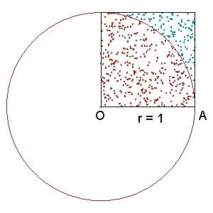
Monte Carlo Method: The Monte Carlo method is a statistical technique used to estimate the value of an unknown quantity using random sampling. In this example, we generate \(N\) random sampling points within a square, and count the number \(h\) of samples that fall in the unit circle. Then the approximation of \(\pi\) is given by: \(4h/N\).

A serial implementation of the Monte Carlo method to approximate Pi may look like the following:

local_count = 0
do i = 1, n_local
    call random_number(x)
    call random_number(y)

    if ((x**2 + y**2) <= 1.0_wp) then
        local_count = local_count + 1
    end if
end do

Parallel Monte Carlo Pi Approximation: To parallelise the Monte Carlo method, we can divide the work among multiple processors. Each processor generates a subset of the total random samples and counts the number of samples that fall within the unit circle. The final approximation of Pi is obtained by summing the counts from all processors and dividing by the total number of samples. See the full code in src/monte_carlo_pi.f90.

Common pitfalls in modern Fortran 

Forgetting implicit none leads to hard-to-find bugs
Mismatched array shapes in assignments or arguments
Missing explicit interfaces when using assumed-shape arrays
Using pointers where allocatables suffice
Overusing save variables (can hide stateful bugs)
Off-by-one indices; arrays default to 1-based indexing